Introduction

One of the most useful concepts that I’ve learned from work is about the beta-binomial model and its bayesian update process. Hence I would like to share this knowledge so that more people can benefit from it.

It is a very easy-to-use technique that can help us overcome the issue of data sparsity and give us a realistic estimation of a probability.

In the context of e-Business, we can use this technique to predict the conversion rate or click-through-rate (number of clicks/number of impressions).

Context for the demo

In the demo below, we will use the click-through-rate (CTR) as an example.

Imagine we just start a business selling books online. When users land on our website, they are exposed to 5 books that were randomly picked from the inventory (and displayed in a random sequence). Each exposure of a certain book is called as one impression. For each book, we might already have a rough intuition about how likely each of these books is likely to be clicked from each impression. However, our intuition might not be accurate enough, so that we will need to rely on the data we collect each day to update the estimation.

In this case, our intuition before collecting any data is called as the prior in Bayesian statistics. With the impression and click data we collect each day after launching the website, we can update the CTR estimation for each book. The final estimation of CTR distribution for each book is also called as the posterior in Bayesian statistics.

Assumptions for the bayesian update process

We treat each impression as a Bernoulli trial with two possible outcomes: success (clicked) vs. fail (not clicked).
Given a CTR probability, the likelihood of observing k clicks out of n impressions is binomially distributed.
Given the number of observed clicks and non-clicks, the CTR estimation is a beta distribution.
Beta distribution is the conjugated prior of Binomial distribution, and the posterior distribution will also be a beta distribution.

Don’t worry if you are not familiar with the concepts like Binomial distribution and Beta distribution.

The demo below will 1) introduce the concepts mentioned above, and 2) walk you through the entire update process with some intuitive visual aids.

More details can also be found in the reference here.

# Import libraries
import numpy as np
import matplotlib.pyplot as plt
import seaborn as sns
%matplotlib inline

What is Binomial distribution?

Given the number of events (e.g., impressions) and its probability (e.g., CTR), a binomial distribution shows the distribution of successes (e.g., clicks).

# n: number of impressions 
impressions = 100 

# p: click-through-rate
CTR = 0.1

# total number of trials
n_trials = 10000

s_binomial = np.random.binomial(impressions, CTR, n_trials)

# final distribution
plt.figure(figsize=(8,6))
plt_binomial = plt.hist(s_binomial)
plt.xlabel('# Clicked cases', fontsize=20)
plt.ylabel('# Trials', fontsize=20)
plt.title('Binomial Distribution: Distribution of successes', fontsize=25);

png

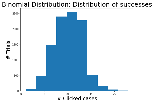
You can see from the chart above in most trails, we have 10 clicks out from 100 impressions as the probability is about 0.1.

What is Beta distribution?

Given the number of successes(alpha: psuedo-clicks) and failures(beta: psuedo-non-clicks), a beta distribution shows the distribution of probability (e.g., CTR).

# Number of clicks
clicks = 20

# Number of non-clicks
non_clicks = 80

# alpha: psuedo-clicks 
alpha = clicks + 1

# beta: psuedo-non-clicks
beta = non_clicks + 1

# Drawn samples from the parameterized beta distribution.
prior_dist = np.random.beta(alpha, beta, size=10000)

plt.figure(figsize=(8,6))
plt_prior_beta = plt.hist(prior_dist)
plt.xlabel('CTR', fontsize=20)
plt.ylabel('# Trials', fontsize=20)
plt.title('Beta Distribution: Distribution of probabilities', fontsize=25);

png

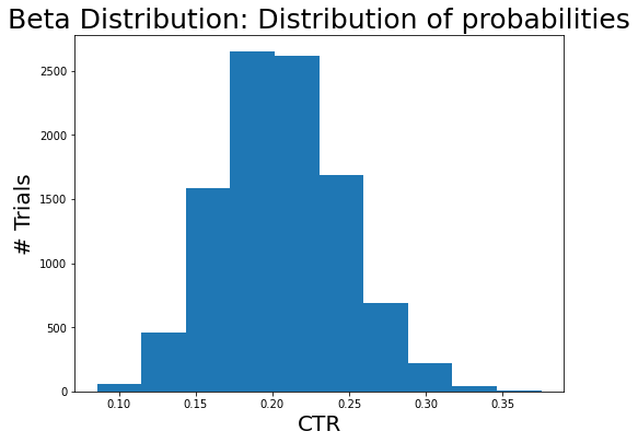
The data indicates that the CTR is likely to be 20% as we saw 20 succeed cases and 80 failed cases.

Beta-binomial model

Let’s do bayesian update in the beta-binomial model now:

According to the reference here, given Binomial likelihood data Bin(obs_impressions, obs_clicks) and a Beta prior Beta(prior_alpha, prior_beta), the posterior distribution should be Beta(prior_alpha + obs_clicks, prior_beta + obs_impressions - obs_clicks).

In order to get the prior_alpha and prior_beta values, we will introduce one more parameter kappa, which indicates the confidence level one has in the prior estimates.

The prior_alpha value should be calculated as prior_CTR * kappa + 1 and the prior_beta should be calculated as (1 - prior_CTR) * kappa + 1.

# Pick a kappa value and prior CTR value
kappa = 100
prior_CTR = 0.1

# Compute prior alpha and beta
prior_alpha = prior_CTR * kappa + 1
prior_beta = (1 - prior_CTR) * kappa + 1

# Compute posterior alpha and beta based on observed data
obs_impressions = 1000
obs_clicks = 40

posterior_alpha = prior_alpha + obs_clicks
posterior_beta = prior_beta + obs_impressions - obs_clicks

# Visualization
prior_dist = np.random.beta(prior_alpha, prior_beta, size=10000)
posterior_dist = np.random.beta(posterior_alpha, posterior_beta, size=10000)

plt.figure(figsize=(8,6))
sns.kdeplot(prior_dist, label='prior')
sns.kdeplot(posterior_dist, label='posterior')
plt.xlabel('CTR', fontsize=20)
plt.legend()
plt.title('Beta-Binomial Bayesian Update', fontsize=25);

png

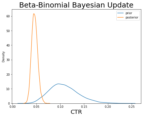
Now we have performed the bayesian update: blue distribution was the prior (i.e., the initial distribution of CTR based on our intuition) and the orange distribution indicates the posterior (i.e., the final distribution of CTR estimation). We usually take the mean or median value of that posterior distribution as the final estimate value of CTR.

In this process, we give the prior CTR estimation a confidence level (i.e., kappa value) and then we update the posterior based on the (impression and click) data we observed.

Also, feel free to change the kappa value in the code above to see how a bigger kappa value will influence the final estimate. Ideally speaking, the higher the kappa values, it requires more data to update the final estimates.

Some more examples: An intuitive illustration of how beta-binomial model deals with data sparsity

# When lacking performance data

prior_alpha = 21
prior_beta = 1001

obs_impressions = 10
obs_clicks = 0

posterior_alpha = prior_alpha + obs_clicks
posterior_beta = prior_beta + obs_impressions - obs_clicks

prior_dist = np.random.beta(prior_alpha, prior_beta, size=10000)

posterior_dist = np.random.beta(posterior_alpha, posterior_beta, size=10000)

plt.figure(figsize=(8,6))
sns.kdeplot(prior_dist, label='prior')
sns.kdeplot(posterior_dist, label='posterior')
plt.xlabel('CTR', fontsize=20)
plt.legend()
plt.title('Bayesian update with little performance data', fontsize=25);

png

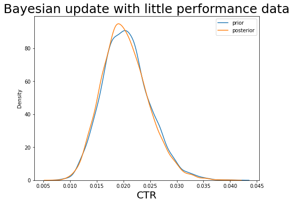
We can see when we do not have data, the posterior distribution is more or less the prior distribution, so that we heavily rely on our intuition.

# When having data

prior_alpha = 20
prior_beta = 1000

obs_impressions = 100000
obs_clicks = 3000

posterior_alpha = prior_alpha + obs_clicks
posterior_beta = prior_beta + obs_impressions - obs_clicks

prior_dist = np.random.beta(prior_alpha, prior_beta, size=10000)

posterior_dist = np.random.beta(posterior_alpha, posterior_beta, size=10000)

plt.figure(figsize=(8,6))
sns.kdeplot(prior_dist, label='prior')
sns.kdeplot(posterior_dist, label='posterior')
plt.xlabel('CTR', fontsize=20)
plt.legend()
plt.title('Bayesian update with more performance data', fontsize=25);

png

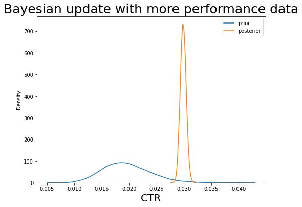
But when we have more performance data, then the posterior distribution is ignoring the info in prior and gives us an estimation mainly based on the performance data.

Conclusion

The beta-binomial model can be implemented in various ways concerning how to pick the prior and kappa values, how to aggregate the performance data, and how many layers of bayesian update one would like to use. It is also very powerful when used together with other machine learning models. I hope this demo helps you to understand the basics of beta-binomial model and how it can be applied in a business context.