Introduction
Time flies, two years have passed since I posted my first blog.
Here I am again, to announce the topic of this year’s first post will be (drumroll, please)…COVARIATE SHIFT!
This was actually inspired by a recent task I had at work. After a couple of weeks of researching, I would like to share a few learnings.
Outline
In this post, two demos are used to explain the issue of covariate shift and to show how to fix it.
In addition, there are two easy quizzes throughout this post to help you check your understanding of the key concepts. You can find the answers to the quizzes at the end of the post.
I have also added a few advanced topics and FAQs (yes, after the summary section, which is prepared for advanced learners).
The source code of all the simulations in the blog post can be found here.
A few more words
Covariate shift is a common issue that data scientists often encounter in the real world. However, not enough attention was paid to it.
At least I was not paying enough attention to this issue before my colleague Alex brought it up. He shared this concept with us using an easy demo (similar to Demo 1 in this post), which helps quite a lot for us to understand the potential issue that we might have at work. So a big thanks to my colleague.
As a machine learning beginner, it is fine if you can grasp the idea of covariate shift and have a basic understanding of how to fix it (as indicated in Demo 1 and 2). The key takeaways will be addressed in the Summary as well.
For those data scientists who already have some hands-on experiences, it is important to have a deeper understanding of this issue:
- Does my model have the issue of covariate shift?
- What are the most-used methods of dealing with covariate shift?
- Any caveats in implementing the covariate shift correction?
Hence, it is recommended to read through the section of the advanced topics and FAQs and check out the simulations.
The FAQs are actually the questions that popped up during the implementation of the covariate shift correction. I was trying to think deeper about questions like 1) whether my dataset indeed has the issue of covariate shift and 2) whether my correction is going to improve the model or make it worse. Hence, I ran a few simulations to solve my own doubts. This part contains my main learnings. I hope it can also help you with your work.
Now, let’s begin the journey!
Hold on, what is covariate shift?
Covariate shift refers to changes in the distribution of features in the training and test dataset.
For those who still have no idea after reading the sentence above, please read the background knowledge session below. Otherwise, please directly go to the first quiz :)
Background knowledge
Warning: Jargon ahead
Training dataset: A set of examples used to fit the parameters of a model.
Test dataset: Dataset used to provide an unbiased evaluation of the model fit on the training data set.
Target: Output variable or dependent variable of the model, the target we want to predict, usually donated by y.
Feature: Input variable or independent variable in the model, it can also be called as covariate, usually donated by x. One model can have one or more features.
Model: a function of feature(s) to predict the target.
What is linear regression?
A simple example of a machine learning model is a linear regression model.
One way to validate a linear regression model is to use Root-Mean-Square-Error, which is also called as RMSE.
The smaller the RMSE, the better the model fits the data.
If you want to know more about linear regression, please feel free to watch the youtube video here.
What is a classifier?
Linear regression is for predicting a continuous target variable.
What if our target variable is a dummy variable (e.g., yes or no)?
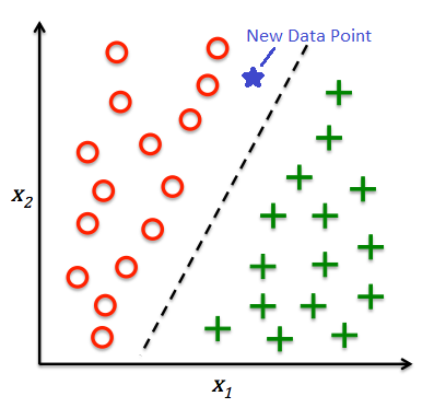
There are also quite a few classification models like logistic regression, multilayer perception classifier.
It is beyond the scope of this session to introduce these concepts in detail.
You just need to know a classifier is a model that predicts a classification problem based on a list of features.
And it is also important to know a few concepts about the validation of a classifier (e.g., confusion matrix, accuracy, precision, and recall):
The higher these scores, the better the model is.
What is covariate shift?
Covariate shift refers to the changes in the distribution of features in the training and test dataset.
It is often called as data drift, feature drift, or population shift.
In the image below (left), we can see that the input density are different between the train and test dataset.
If we train a model using the training samples (i.e., blue dots in the right pic), we will get an inaccurate model for predicting the test sample (i.e., black dots in the right pic).

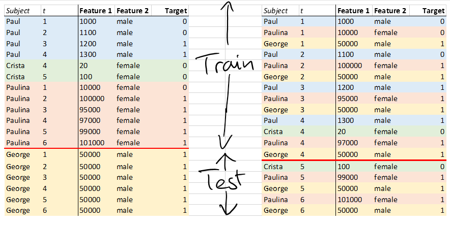
Quiz 1: Which example below (left vs. right) is more likely to have the issue of covariate shift?
You can find the answer at the end of this post.
What is covariate shift correction?
The key idea behind the covariate shift correction is to train a re-weighted model.
It puts more weight on the samples with feature values that are more frequently shown in the test set, and vice versa.
You might wonder how to calculate the weight, so here come two demos:
- Demo 1: a simple example with only one feature in the dataset and it provides an intuitive solution
- Demo 2: an example with two features and uses a more general approach to correct for the covariate shift
Demo 1: An intuitive example with one feature only
Data Preparation
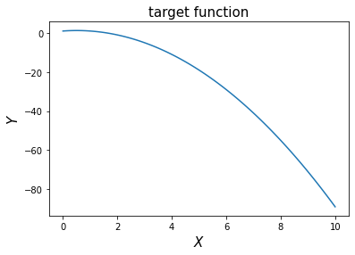
Prepare a target function with only 1 feature
Let us assume the relationship between x and y is as following: \[f(x) = -x^2 + x + 1\]
Prepare the train and test dataset (n=1000)
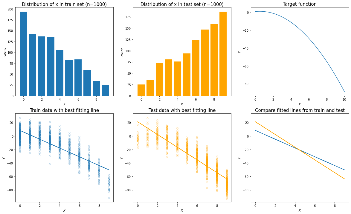
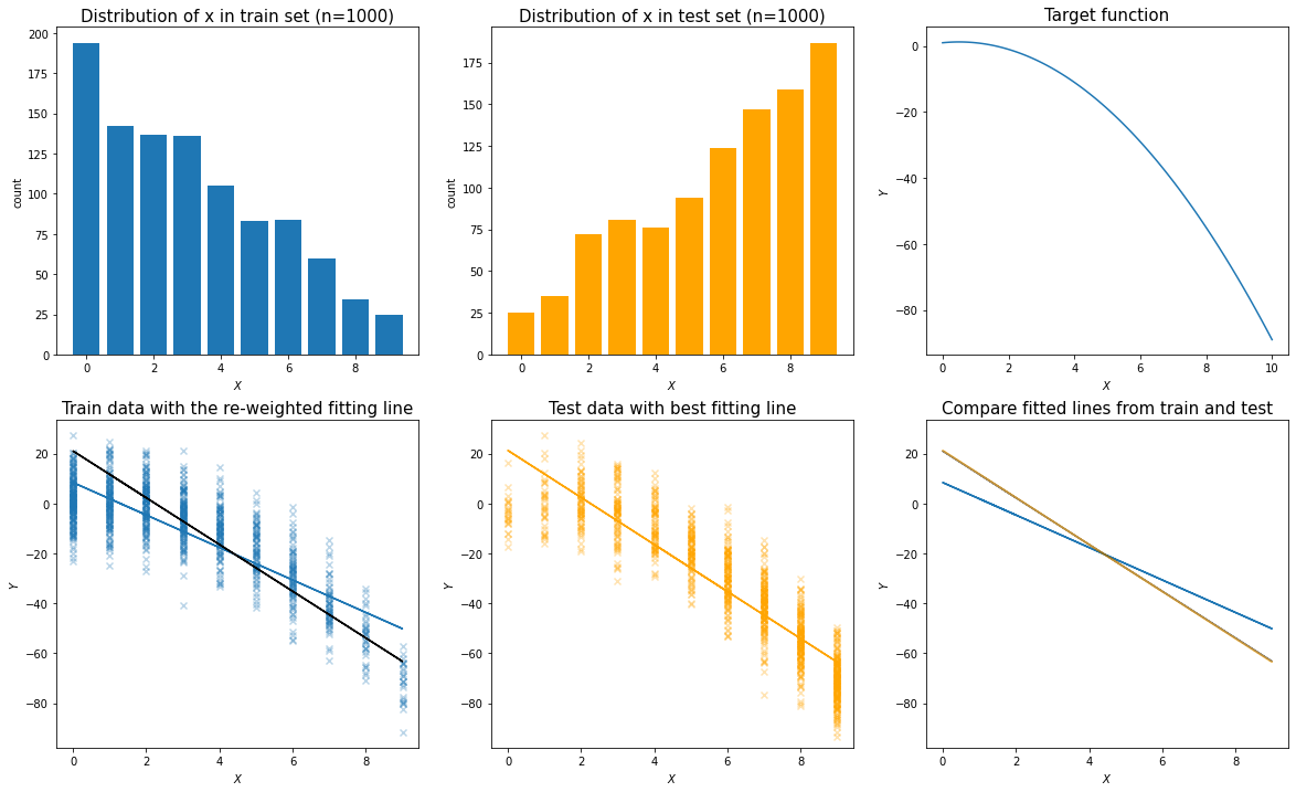
Then we generate the two sets of x distributions for training and test set (see the first two charts below).
Hence, the train and test data were generated by adding some random error on top of the expected y value for each x.
Visualize covariate shift
Let’s try to find the besting fitting line for the train and test data respectively. In the last chart below, we can see that the best fitting lines from the training and the test set are different from each other.
An intuitive solution
Remember that our goal is to generate an accurate model for the test data.
When there is a big difference in the feature distribution between the train and test dataset, we need to correct it by adjusting the weight of samples in the test set.
But how can we find the best weight to apply?
Intuitively speaking, we should use the ratio of the probability distribution of x: P_test(x)/P_train(x)
We already know the probability distribution of the feature in the train and test dataset.
P_train(x):
| x | frequency | p | |
|---|---|---|---|
| 0 | 0 | 194 | 0.194 |
| 1 | 1 | 142 | 0.142 |
| 2 | 2 | 137 | 0.137 |
| 3 | 3 | 136 | 0.136 |
| 4 | 4 | 105 | 0.105 |
| 5 | 5 | 83 | 0.083 |
| 6 | 6 | 84 | 0.084 |
| 7 | 7 | 60 | 0.060 |
| 8 | 8 | 34 | 0.034 |
| 9 | 9 | 25 | 0.025 |
P_test(x):
| x | frequency | p | |
|---|---|---|---|
| 0 | 0 | 25 | 0.025 |
| 1 | 1 | 35 | 0.035 |
| 2 | 2 | 72 | 0.072 |
| 3 | 3 | 81 | 0.081 |
| 4 | 4 | 76 | 0.076 |
| 5 | 5 | 94 | 0.094 |
| 6 | 6 | 124 | 0.124 |
| 7 | 7 | 147 | 0.147 |
| 8 | 8 | 159 | 0.159 |
| 9 | 9 | 187 | 0.187 |
Quiz 2: Which weight below is the correct one?
Option A: putting more weights when x is smaller
| x | weight | |
|---|---|---|
| 0 | 0 | 7.760000 |
| 1 | 1 | 4.057143 |
| 2 | 2 | 1.902778 |
| 3 | 3 | 1.679012 |
| 4 | 4 | 1.381579 |
| 5 | 5 | 0.882979 |
| 6 | 6 | 0.677419 |
| 7 | 7 | 0.408163 |
| 8 | 8 | 0.213836 |
| 9 | 9 | 0.133690 |
Option B: putting more weights when x is larger
| x | weight | |
|---|---|---|
| 0 | 0 | 0.128866 |
| 1 | 1 | 0.246479 |
| 2 | 2 | 0.525547 |
| 3 | 3 | 0.595588 |
| 4 | 4 | 0.723810 |
| 5 | 5 | 1.132530 |
| 6 | 6 | 1.476190 |
| 7 | 7 | 2.450000 |
| 8 | 8 | 4.676471 |
| 9 | 9 | 7.480000 |
Fit the best line in the train set after re-weighting and visualize
Now we can see the best fitting line after re-weighting (the black line in the left bottom chart) is overlapping with the best fitting line for the test data (the orange line in the right bottom chart).
The re-weighted model performs better than before regarding the test sample.
Demo 2: What shall we do if there is more than 1 feature?
Data Preparation
Prepare a target function with 2 features
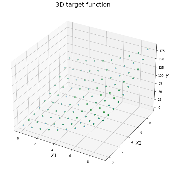
Prepare train and test data (n=1000) and visualize
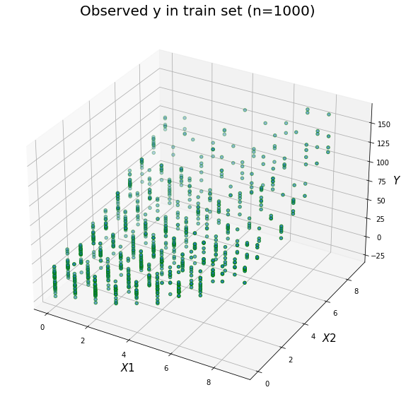
| x1 | x2 | y | |
|---|---|---|---|
| 0 | 4 | 6 | 67.714352 |
| 1 | 4 | 3 | 21.090243 |
| 2 | 2 | 6 | 63.327070 |
| 3 | 3 | 2 | 15.873481 |
| 4 | 3 | 4 | 25.794113 |
| ... | ... | ... | ... |
| 995 | 0 | 1 | 5.721640 |
| 996 | 2 | 0 | 16.315458 |
| 997 | 1 | 5 | 36.275323 |
| 998 | 1 | 4 | 30.408138 |
| 999 | 0 | 4 | 12.980950 |
1000 rows × 3 columns
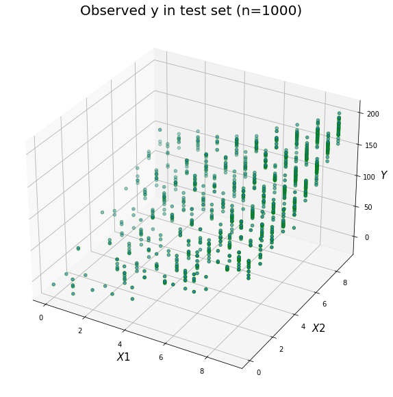
| x1 | x2 | y | |
|---|---|---|---|
| 0 | 5 | 9 | 125.714352 |
| 1 | 9 | 9 | 169.090243 |
| 2 | 6 | 7 | 113.327070 |
| 3 | 3 | 5 | 39.873481 |
| 4 | 8 | 8 | 137.794113 |
| ... | ... | ... | ... |
| 995 | 3 | 5 | 45.721640 |
| 996 | 0 | 9 | 100.315458 |
| 997 | 7 | 5 | 90.275323 |
| 998 | 8 | 1 | 82.408138 |
| 999 | 6 | 3 | 46.980950 |
1000 rows × 3 columns
Covariate shift correction in four steps
With the following four steps, you can easily do the covariate shift correction.
Step 1: concatenate train (label 0) and test data (label 1)
Step 2: train a classifier between train and test (could be logistic regression or multilayer perceptron classifier)
Step 3: calculate the density ratio (p1/p0) for the train set
Step 4: train the model with the weighted sample (using density ratio as the weight)
Finally, as a validation, we will compare the RMSE of train and test data using different model results to see the effect of the correction.
Step 1: concatenate train (label 0) and test data (label 1)
# Step 1: assign a label of 1 to test data set, and a label of 0 to train data set
df_test["label"] = 1
df_train["label"] = 0

# Concat the two datasets into one data set
df_combined = pd.concat(
    [df_train[["x1", "x2", "label"]], df_test[["x1", "x2", "label"]]]
)

df_combined
| x1 | x2 | label | |
|---|---|---|---|
| 0 | 4 | 6 | 0 |
| 1 | 4 | 3 | 0 |
| 2 | 2 | 6 | 0 |
| 3 | 3 | 2 | 0 |
| 4 | 3 | 4 | 0 |
| ... | ... | ... | ... |
| 995 | 3 | 5 | 1 |
| 996 | 0 | 9 | 1 |
| 997 | 7 | 5 | 1 |
| 998 | 8 | 1 | 1 |
| 999 | 6 | 3 | 1 |
2000 rows × 3 columns
Step 2: train a classifier between train and test
Train the classifier:
# Step 2: train the classifier using the combined dataset
X = df_combined[["x1", "x2"]]
y = df_combined["label"]

## Train logistic regression
clf = LogisticRegression().fit(X, y)
df_combined["label_hat_lr"] = clf.predict(df_combined[["x1", "x2"]])
Check the accuracy of the classifier:
def check_accuracy(df, col_y_pred, col_y_true="label"):
    accuracy = accuracy_score(df[col_y_true], df[col_y_pred])
    precision = precision_score(df[col_y_true], df[col_y_pred])
    recall = recall_score(df[col_y_true], df[col_y_pred])
    print(
        f"""
            accuracy: {round(accuracy, 3)}
            precision: {round(precision, 3)}
            recall: {round(recall, 3)}
    """
    )
    return accuracy, precision, recall

check_accuracy(df_combined, "label_hat_lr")
Results:
accuracy: 0.794
precision: 0.799
recall: 0.786
Step 3: calculate the density ratio (p1/p0) for the train set
# Step 3: get the density ratio for training set
df_train["density_ratio"] = [
    i[1] / i[0] for i in clf.predict_proba(df_train[["x1", "x2"]])
]

df_train
| x1 | x2 | y | label | density_ratio | |
|---|---|---|---|---|---|
| 0 | 4 | 6 | 67.714352 | 0 | 1.633294 |
| 1 | 4 | 3 | 21.090243 | 0 | 0.433734 |
| 2 | 2 | 6 | 63.327070 | 0 | 0.758671 |
| 3 | 3 | 2 | 15.873481 | 0 | 0.190007 |
| 4 | 3 | 4 | 25.794113 | 0 | 0.459901 |
| ... | ... | ... | ... | ... | ... |
| 995 | 0 | 1 | 5.721640 | 0 | 0.038664 |
| 996 | 2 | 0 | 16.315458 | 0 | 0.053502 |
| 997 | 1 | 5 | 36.275323 | 0 | 0.332354 |
| 998 | 1 | 4 | 30.408138 | 0 | 0.213626 |
| 999 | 0 | 4 | 12.980950 | 0 | 0.145596 |
1000 rows × 5 columns
Step 4: Trian models using density ratio
def compute_rmse(df_train, df_test, weight=None):
    X = df_train[["x1", "x2"]]
    y = df_train["y"]
    if weight:
        w = df_train[weight]
        # train a weighted model
        lr = LinearRegression().fit(X, y, w)
        df_train[f"y_hat_{weight}"] = lr.predict(X)
        df_test[f"y_hat_{weight}"] = lr.predict(df_test[["x1", "x2"]])
        print("RMSE for train set:")
        print(round(rmse(df_train["y"], df_train[f"y_hat_{weight}"]), 2))
        print("")
        print("RMSE for test set:")
        print(round(rmse(df_test["y"], df_test[f"y_hat_{weight}"]), 2))

    else:
        # train simple linear regression
        lr = LinearRegression().fit(X, y)
        df_train[f"y_hat"] = lr.predict(X)
        df_test[f"y_hat"] = lr.predict(df_test[["x1", "x2"]])
        print("RMSE for train set:")
        print(round(rmse(df_train["y"], df_train["y_hat"]), 2))
        print("")
        print("RMSE for test set:")
        print(round(rmse(df_test["y"], df_test["y_hat"]), 2))
    return df_train, df_test, lr
Validation: Compare RMSE across models
No correction: simple linear regression
df_train, df_test, lr = compute_rmse(df_train, df_test)
RMSE for train set:
167.65

RMSE for test set:
352.05
With correction: weighted linear regression using density ratio
df_train, df_test, weighted_lr = compute_rmse(df_train, df_test, "density_ratio")
RMSE for train set:
280.07

RMSE for test set:
168.52
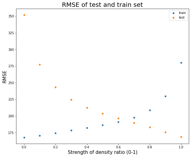
Adjusting the intensity of the density_ratio
The results above indicated that making the correction will increase error in the training set, but reduce error in the test set. What if we adjust the strength of the density ratio as a weight for the main model. You can find the simulation result below:
Summary
Covariate shift
Covariate shift refers to the changes in the distribution of features in the training and test dataset.
Covariate shift correction: importance weight using density ratio
The key idea behind the general approach of covariate shift correction is to train a classifier between the training and test set.
Then we can get the density ratio of p_test(x)/p_train(x) and use it to reweight the training set for training the final model.
Notes:
-
p_train(x): the probability of a sample comes from the training dataset given a set of features
-
p_test(x): the probability of a sample comes from the test dataset given a set of features
-
density ratio: p_test(x)/p_train(x)
Challenges?
Although the demos in this notebook seem promising and easy to implement, the application of covariate shift correction in the real world is still questionable:
- Need to have knowledge of the test data
- Need to have some knowledge of the target function
- Need to identify if there is a covariate shift or not
- Training the classifier is very time consuming for high-dimension dataset
- Uncertain results: It is possible that using a model that corrects for covariate shift may produce worse results than using a standard model without the correction.
Advanced topics
More background knowledge:
Types of dataset shift: Covariate shift (the shift of feature distributions) is not the only dataset shift we are likely to encounter, there are more types of dataset shift:
- prior probability shift: the shift of the target distribution
- concept shift: the shift of the relationship between the target and the feature(s)
- domain shift: involves changes in measurement
How to identify covariate shift?
- visualize feature distribution
- train a classifier for the combined data method (check for each feature)
Two methods of dealing with covariate shift:
- dropping of drifting features
- importance weight using density ratio estimation
- train a classifier yourself
- use a package like densratio to get density ratio
Frequently asked questions:
Q1: What if the classifier model is not accurate enough?
Answer:
- Situation 1: There is not too much signal in distinguishing train and test set –> no need to do covariate shift correction
- Situation 2: The classifier is not good enough to describe the feature difference between test and train set –> improve the classifier (e.g., instead of using logistic regression, use Multi-Layer Percepton)
Simulation:
In this simulation, we are going to reuse the datasets in Demo 2 and train a less accurate classifier by reducing the number of features.
# Bonus test: train a "poor" classifier using less features
X1 = df_combined[["x1"]]
y = df_combined["label"]

## Train logistic regression
clf1 = LogisticRegression().fit(X1, y)
df_combined["label_hat_lr_1"] = clf1.predict(df_combined[["x1"]])

print("Check the accuracy of the calssifier: logistic regression with only 1 feature")
display(_=check_accuracy(df_combined, "label_hat_lr_1"))
Check the accuracy of the “poor” classifier:
    accuracy: 0.706
    precision: 0.709
    recall: 0.696
Make correction and check RMSE for train and test data:
# prepare the correct version of density ratio using the logistic regression model
df_train["density_ratio_1"] = [
    i[1] / i[0] for i in clf1.predict_proba(df_train[["x1"]])
]

df_train, df_test, weighted_lr_1 = compute_rmse(df_train, df_test, "density_ratio_1")
RMSE result with a poor classifier (trained with 1 feature):
  RMSE for train set:
  219.39

  RMSE for test set:
  240.58
When we compare this result with the RMSE values above, we can see the weak classifier did the correction somehow, but the result is not as good as the result of a good classifier.
Q2: What if the sample size in the train set does not equal to the sample size in the test set?
**Answer: **
It is no problem when using the approach in the first demo (see simulation below).
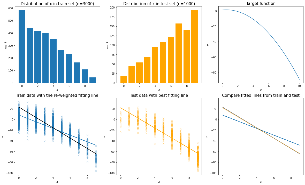
However, when training the classifier as in the second approach, it is not recommended to use p_test(x)/p_train(x) directly, as it will result in a list of density ratios that are not centered at the value of 1.
Two solutions:
- Resample the training or test set to make the sample sizes equal
- After getting the density ratio, adjust it based on the sample size ratio (n_test/n_train)
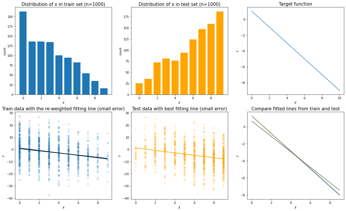
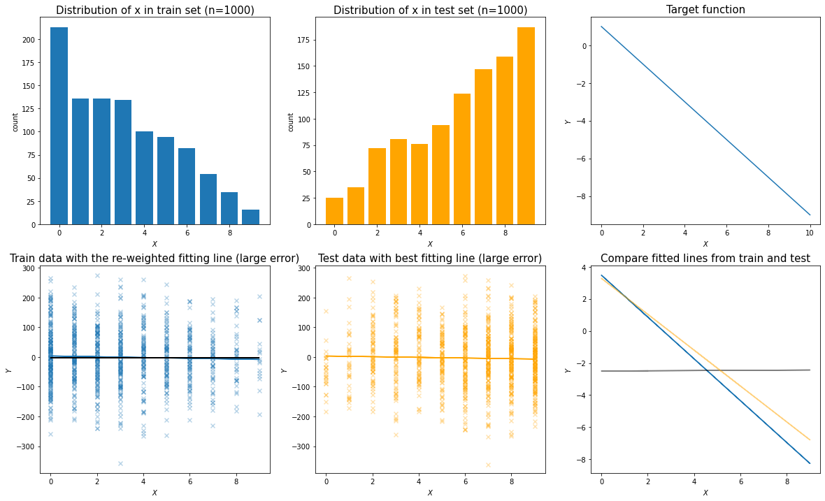
Q3: What if the target function is perfectly linear?
Answer:
There is no need to do covariate shift correction if the target function is perfectly linear and the main model is also linear.
- Situation 1: When the error term in the observed data is relatively small, there should be no impact.
- Situation 2: When the error term in the observation data is large, then the prediction bias is mainly from the error term in the train and test data. The covariate shift correction will not work as well.
Simulation for Situation 1: relative small error term when generating the simulation data
Simulation for Situation 2: relative large error term when generating the simulation data
Quiz answers
Answer to Quiz 1: Left
Answer to Quiz 2: Option B
References
http://iwann.ugr.es/2011/pdf/InvitedTalk-FHerrera-IWANN11.pdf
https://www.youtube.com/watch?v=24YZ_62Jn-o&ab_channel=AlexSmola